Graphing Lines Worksheets
About These 15 Worksheets
Graphing Lines Worksheets are educational tools designed to help middle school students understand and master graphing lines on a coordinate plane. As students begin working with graphs, it’s important they understand coordinate plane quadrants, which divide the grid into sections and help locate points accurately. These worksheets include a range of exercises that build step by step, starting with basic graphing skills and moving toward more advanced concepts.
The basic idea behind graphing lines is that you’re taking an equation, like y = 2x + 3, and drawing it on a coordinate plane. This graph visually represents all possible solutions to the equation. The coordinate plane, as you may already know, is a two-dimensional space defined by a horizontal axis (x-axis) and a vertical axis (y-axis). A line graphed on this plane provides a visual representation of a relationship between two variables – the x (independent variable) and y (dependent variable).
The Types of Exercises on These Worksheets
The collection of graphing lines worksheets forms more than a progression of mathematical exercises-they’re a gradual deepening of spatial reasoning, symbolic thought, and pattern recognition. What begins as mechanical plotting evolves into conceptual understanding and even reflection on how we perceive and express relationships in space.
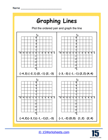
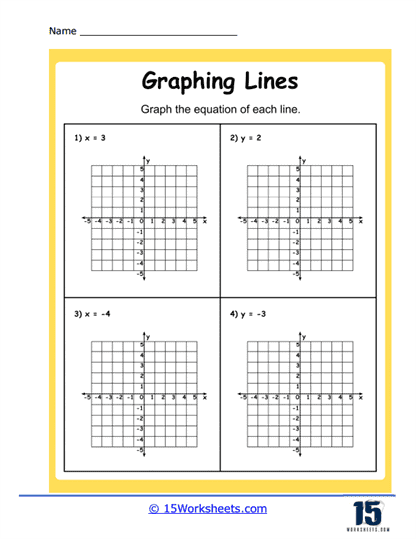
In Putting Points Together, students begin by learning that each point, seemingly isolated on a grid, can connect to others in meaningful, predictable ways. The act of linking those dots isn’t just about forming lines-it’s about discovering that two numbers can tell a story. That story becomes richer in Simple Lines, where students plot and draw basic linear graphs, slowly absorbing that change isn’t random; it has direction and consistency. Points From Equations builds on this by showing that equations aren’t just abstract rules-they generate those points. A student writing x = 2 and y = 2x + 3 isn’t just solving a problem; they’re creating structure, sketching the invisible architecture of relationships between variables.
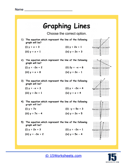
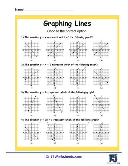
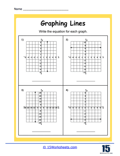
As students begin to see the shape of these relationships, the worksheets ask for interpretation. In Explain the Line, learners give voice to the graphs-what kind of change is represented, what the graph is doing, and why it matters. Equations and Lines challenges them to pair visual patterns with symbolic expressions, solidifying that the two speak the same language. Write the Equation reverses the process-given a line, students must translate it back into its algebraic identity. Each of these worksheets reinforces a central idea: math isn’t about plugging in numbers, but about understanding how ideas are mapped, mirrored, and transferred between different forms.
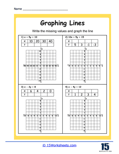
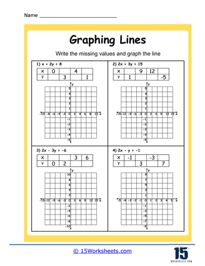
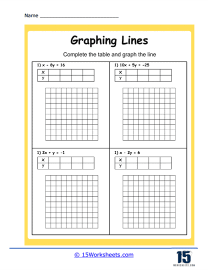
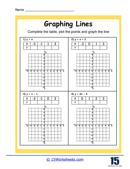
Once that foundation is laid, the worksheets begin to introduce uncertainty, asking students to find the missing pieces in Missing X and Y. There is something quietly powerful in being asked to restore a broken structure-figuring out the absent values is no longer guesswork but an act of logic grounded in consistent rules. In Complete the Table, students see how a pattern expands across a set of inputs, moving from static calculations to a deeper appreciation of regularity and flow. Tables become another kind of map, not just a box of values, but a cross-section of change.
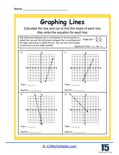
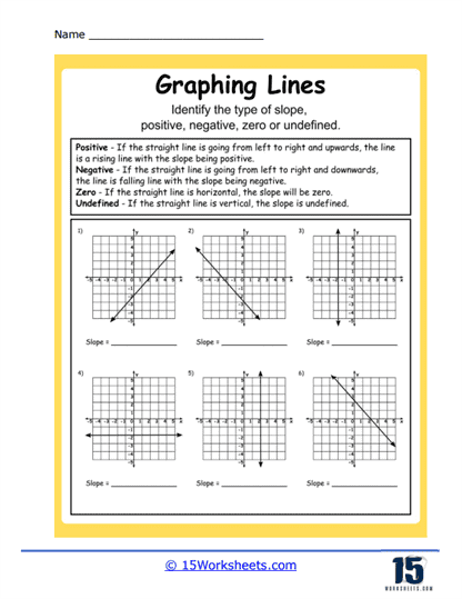
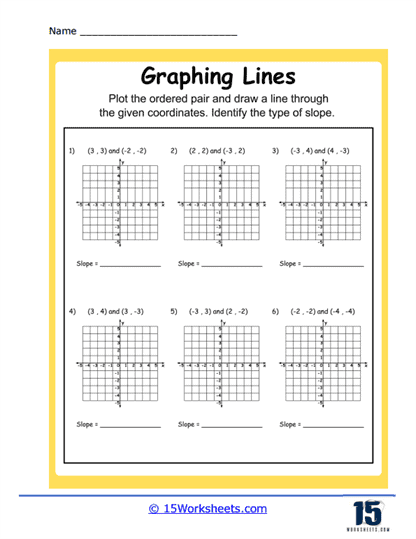
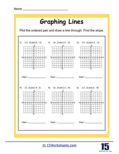
The heart of graphing lines is slope-the rate at which one variable changes in relation to another-and several worksheets slow down to focus on this crucial concept. Using Slope is where students begin to measure movement rather than just observe it. In Explaining Slope, they are asked not just to calculate but to reason: why does this value matter? How does it alter the line’s behavior? In Slope of Points, they apply this across pairs of coordinates, observing how position and difference are tied together. 2-Point Lines Worksheet then weaves these skills into a complete task-two points, one line, a slope, an equation-showing how all parts of the system are mutually dependent.
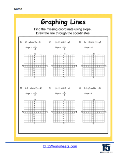
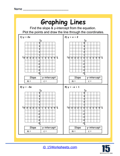
By this stage, the worksheets demand full synthesis. Complete the Line Equation gives only part of the story, asking students to infer what’s missing using the information they have. Slope and Intercept asks them to extract structure from raw information-find the rise, find the starting point, and reconstruct the rule. y-Coordinates brings the focus to prediction: given a rule and a new input, what outcome should you expect? The student is no longer plotting or interpreting-they are anticipating, foreseeing, using what they know to project what they do not yet see.
How to Graph a Linear Equation
Graphing a linear equation can seem like a daunting task if you’re not familiar with the process, but once you understand the steps involved, it becomes straightforward. Let’s break it down.
A linear equation is an equation between two variables that produces a straight line when graphed. These equations are typically written in the form y = mx + b, where m represents the slope of the line and b is the y-intercept. Here’s a step-by-step guide on how to graph a linear equation:
1. Identify the Slope and the y-intercept – Start by rewriting your equation in slope-intercept form (y = mx + b) if it’s not already in that form. In this form, m is the slope of the line, and b is the y-intercept.
For example, in the equation y = 2x – 3, the slope (m) is 2, and the y-intercept (b) is -3.
2. Plot the y-intercept – The y-intercept is the point where the line crosses the y-axis. This is always the point (0,b). Start by finding the y-intercept on your graph and make a point at this location.
In our example, the y-intercept is -3. So, plot a point at (0, -3).
3. Use the Slope to Plot the Next Point – The slope is a measure of the steepness of the line and is defined as the ratio of the vertical change (the rise) to the horizontal change (the run). If the slope is positive, the line rises from left to right, and if it’s negative, it falls from left to right. If the slope is 2, for example, this means you go up 2 units (rise) for every 1 unit you go to the right (run).
In our example, the slope is 2. Starting from the y-intercept, count 2 units up (rise of 2) and 1 unit to the right (run of 1), and then make a point there.
4. Draw the Line – Once you have at least two points, you can draw a line that passes through them. This line is the graph of your linear equation. You can extend the line as far as you want in both directions, but be sure to draw arrows on the ends of the line to indicate it extends indefinitely.
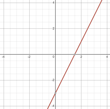
In our example, you should have a line passing through the points (0, -3) and (1, -1).
Remember to label your graph, indicating the equation of the line, and the x and y axes.
Understanding how to graph a linear equation is a fundamental skill in algebra. It helps you visualize the solutions to the equation and the relationship between the variables. Additionally, it aids in understanding more complex mathematical concepts like systems of equations and inequalities.
Real-life applications of graphing linear equations are abundant in various fields such as physics, economics, and engineering. For instance, businesses often use linear equations to predict future sales based on past data, and engineers use them to model and solve problems involving constant rates of change.
By learning to graph a linear equation, you’re not only gaining a key mathematical skill but also equipping yourself with a tool that can help solve real-world problems and make informed decisions based on trends and predictions.